How a kids' novel inspired me to simulate a gene drive on 86 million genealogy profiles

I read a novel where the rules for inheriting witchcraft resembles the real-world gene drive, so I developed a simulation and queried 86 million genealogy profiles to see how witchcraft would spread in real life.

Table of Contents

1. Introduction: all my hobbies combined
2. The theory behind gene drives
3. Estimating gene drive behaviour with a mathematical model
4. Simulation
5. Importing the Familinx dataset
6. Why is my SQL index slowing down my query?
7. First look at the Familinx data
8. Marking all descendants with breadth-first search
9. Analysing the Familinx dataset
10. Conclusion
11. What I learned
12. What I need to learn next

Introduction: all my hobbies combined

This blog post combines my two hobbies: programming and reading kids’ books. (No, really.)

You might think I’m immature because I’m an adult reading kids’ books. I disagree. Middle-grade books (novels written for 9-12 year olds) distill a wide variety of topics, human nature, and life lessons into a short and concise format: I can finish one in just one afternoon, learning new things and acquiring fresh ideas along the way. So no, I’m not being childish: I’m being efficient!

Recently, I’ve been eagerly awaiting Stephanie Burgis’ new middle-grade book, The Girl with the Dragon Heart, which finally came out this week. It’s about how a well-told story can change the world: the main character is a young, intelligent, independent… public relations expert. I first encountered this character in the previous book, The Dragon with the Chocolate Heart, where she’s the best friend of the main character. Her portrayal singlehandedly changed my view on PR people from shadowy manipulators to skilled experts who uses words to make allies and help people achieve their goals. I couldn’t wait to read more about her story.

I also enjoyed Chocolate Heart because its story paralleled my own life at the time. That book follows a young dragon’s journey to find her purpose in life, and how she learns to recover from failure with the help of her new friends, her family, and delicious chocolate. When I found this book earlier this year, I was also trying to find my place in life and looking to turn my passion with computers into a career. The book’s main character’s story gave me the courage to start this very blog.

However, my favorite middle-grade series by Burgis is the Kat, Incorrigible series, a delightful trilogy set in an alternate Regency England with magic. It features Kat, a spirited clever young woman whose plans to help her family always gets her into hilarious scrapes. She learns that the bond of siblings is more powerful than any sinister magic. The books are all entertaining, witty, and unique: It’s the only book I’ve read that sets up a trope then subverts it in the first two sentences.

I’m fascinated by magic in books, because I’ve always wanted to solve problems by whispering a few arcane words, and there’s nothing like that in real life. (Nope, none at all.) And the rule for inheriting magic in Kat, Incorrigible was especially interesting.

In Kat’s world, all the children of a witch inherits witchcraft. So if either your father or mother have witchcraft powers, then you’ll also have witchcraft powers. This is different from how heredity works in real-life, where most traits from a parent aren’t guaranteed to be passed on to a child.

One of the Kat books mentions that, in 1809, about 5% of the population have witchcraft powers. That seemed too low: if each parent with witchcraft will produce multiple witch children, shouldn’t the proportion of witches grow exponentially?

I did some research: it turns out this inheritance pattern is very similar to the real-life gene drive.

The theory behind gene drives

A gene drive refers to any genetic engineering technology that bypasses the normal rules of inheritance to spread a particular trait.

Usually, an allele (a variation of a gene) only has a 50% chance of being inherited by any offspring. With gene drives, this chance is increased - up to 100% of children inherits the gene. Then all their children’s children inherits the gene, and so on, resulting in the gene rapidly spreading through the population.

Researchers have tested gene drives for disease control, mostly against mosquitos. For example, a 2015 study used a CRISPR/Cas9-based gene drive to quickly spread the gene for malaria resistance in a mosquito population. Just last month, a new study used CRISPR/Cas9 to make all female offsprings of mosquitos sterile, eliminating an entire mosquito population in only seven generations.

Hmm. If a parent has the gene drive, then all their children will inherit the gene drive. Doesn’t that sound exactly like the rule for inheriting witchcraft in Kat’s world? This means we can model witchcraft inheritance as a gene drive.

Estimating gene drive behaviour with a mathematical model

Researchers from Cornell University, led by Robert Unckless, published equations for estimating how fast a gene drive would spread.

They started with the standard Wright-Fisher population model, which has two assumptions:

• A population’s size is constant
• Anyone in the population can mate with any other member.

The Unckless paper then adapted the Wright-Fisher estimates to show that a gene drive grows exponentially. In addition, they came up with a formula to calculate how long it takes for a gene drive to spread, given the starting percentage of population with the gene drive.

I plugged five initial ratios into their formula: 1%, 5%, 10%, 15%, 20%. (5%, if you recall, is the estimated prevelance for witchcraft given in the books). See Appendix A for the calculations.

Here’s the time to half results for each starting ratio:

q0=1% generations to half: 9.711785734104552 or 252.50642908671836 years
q0=5% generations to half: 8.907066777887502 or 231.58373622507506 years
q0=10% generations to half: 8.56049318760753 or 222.5728228777958 years,
q0=15% generations to half: 8.357760633553447 or 217.30177647238963 years
q0=20% generations to half: 8.213919597327557 or 213.5619095305165 years

In summary, it should take about 8 to 9 generations, or about 200-250 years, for half the population to carry the witchcraft trait. Easy!

However, Unckless cautions that their theory, in addition to inheriting simplications from the Wright-Fisher model, has one additional limitation: it assumes that S_e, the selection coefficient, is small. The selection coefficient for my witchcraft gene is very large (S_e = 1), so how does that affect the result?

I wrote a simulation to find out.

Simulation

I made a simulation to validate the theory’s predictions.

The simulation needs to match the assumptions of the Wright-Fisher model. This means a constant population size with random pairing.

The implementation (simulate_const) is super naive and simple. I first allocate an array of 2726150 elements, and then adds the gene drive trait to the desired initial proportion of elements.

Now, for each generation:

1. I shuffle the list of people.

2. I simulate mating between adjacent pairs of elements.

Each pair will produce two children (to keep the population constant). If either parent has the gene drive trait, then both of their children will get the trait.

3. I repeat the above two steps with the new generation of offspring.

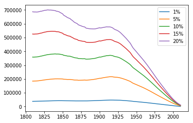
Here’s the simulation results for starting ratios of 1, 5, 10, 15, and 20 percent:

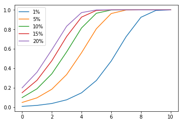
In the simulation, the proportion of people with the gene drive trait did grow exponentially, as predicted, but it rose way faster than expected. For example, the 5% simulation reached 50% ratio in about 4 generations, way faster than the 8.9 generations estimated by Unckless’s formula.

This does confirm my suspicion: since our selection coefficient is very high (100%), we’ve violated the formula’s assumption of low selection coefficient, so the formula will always underestimate how fast the gene drive spreads.

Simulations are easy to tweak, so trying new scenarios is simple (see Appendix B). But I don’t want to just analyze simulations: I want real world data. Fortunately, I discovered a huge open dataset of 86 million genealogy records that, at least initially, sounded perfect for this investigation.

Importing the Familinx dataset

The Familinx dataset is an open dataset released earlier this year that contains 86 million anonymized genealogy records.

When I heard about it, I was excited: I could run my simulation on the family trees from this real dataset to validate my simulations and estimates.

I downloaded the dataset from Familinx’s website, and received two files:

• a 16GB list of profiles containing metadata such as birth year, death year, and place of birth for all 86 million people in the dataset

• and a 170MB relations file, where each line contains two numbers: the ID of a parent, and the ID of their child.

This results in a directed graph, where the nodes are in one file, while the edges are in the other.

Since I want to find out how the population would change over time, I first need to count how many people are alive in each year in the data.

For this task, I only needed to look at the profiles, not the relations. To filter a table of 86 million rows based on criteria, I decided to load the profiles into an SQL database, which is optimized for such queries. I chose the popular and free PostgreSQL database.

First, I used PostgreSQL’s COPY command to load the Familinx dataset’s list of profiles into the database.

Next, I formulated my query: a person is alive in the current year if:

• they were born before or during this year

and

• they didn’t die before this year.

The query also must ignore entries with invalid data - profiles with no birth year, no death year, or an invalid birth year.

Taking all that into account, this is my query to count how many people are alive during 1809:

select count(1) from profiles where birth_year is not null and death_year is not null
and birth_year > 1700 and birth_year <= 1809 and death_year >= 1809;

After a minute of processing, psql outputs:

  count  
---------
 2726151
(1 row)

Cool: I now know this dataset contains 2.7 million people who were alive during 1809.

However, I need to run this for all years I care about in the dataset - that’s 1800 to 2010. 210 years, each taking one minute to query = 210 minutes, or 3 and a half hours. I also wanted to query some other things, so that’s going to take an entire day.

Can I speed that up?

Why is my SQL index slowing down my query?

I only took one database course, Stanford’s free online db-class back in 2011, which didn’t cover optimizations. Since I didn’t know what I was doing, I decided to just unthinkingly parrot advice and create an index on the two columns I’m querying. I figured an index can’t make performance worse, right?

create index profiles_birth_and_death_years on profiles (birth_year, death_year);

I rerun the same query, and… after 10 minutes, the query’s still not done. Adding a query actually slowed the query down.

A check with the EXPLAIN command confirms that the query is using the index. So why is it so much slower now?

Markus Winand’s great site on SQL indexes explains where my assumptions don’t match reality.

An index speeds up the process of finding all records with a matching value in the indexed columns. Then, the database only has to process that set of records with duplicate values instead of the entire dataset. This works very fast if the data doesn’t have many duplicate values in the indexed columns.

However, many people share a birth year and death year, so the database needs to process many duplicate values after the index lookup. In addition, because my search criteria is not checking for one equality, but a range of dates, the database must look up all years less than my queried year in the index. This requires the database to visit almost all the data anyways, but now with the added overhead of an index query.

Thus, an index doesn’t fit my use case, and that’s why it actually made the query slower. Now I understand why Database Administrators earn such high salaries.

Instead of trying to optimize the query, I simply ran my computer overnight, getting my results in the next day.

(I also tweaked the query for years after 1900: the new query accounts for people who do not have a death year because they are still alive today. This modified query is used for all years after 1900 in the rest of this experiment.)

First look at the Familinx data

Here’s the number of people alive during each year in the dataset, from 1800 to 2010:

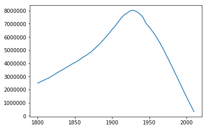
Like the world’s population as a whole, the population in the dataset grows - until 1950-ish, when the population suddenly drops. I guess this happens because people born after 1950-ish are too young to conduct genealogies, so they would be underrepresented in the database.

OK, so maybe this data isn’t representative of the real world population after 1950. Is it representative for years before 1950? I decided to calculate the male/female ratio for each year: if this subset of the population is a good sample of the general population, then I would expect the male/female ratio to match the global ratio, 50%.

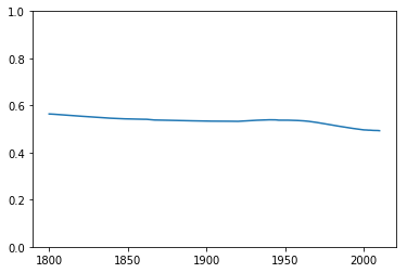
The ratio stays constant around 50%, showing that in this respect this data is a good representation of the population as a whole.

Marking all descendants with breadth-first search

I simulated the effect of a gene drive on the Familinx data with two steps:

First, I queried the list of people alive in 1809, and picked a subset of them (1, 5, 10, 15, or 20% of them) as carriers of the gene drive.

Next, I looked for all their descendants in the relations file. To do this, I used a modified flood fill with a queue implementing a breadth-first traversal.

To illustrate this without graphing like 86 million nodes, here’s a small placeholder family tree.

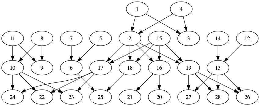
Each person is assigned a numerical ID, because that’s how anonymized Familylinx data identifies each individual. (Also, for this made-up example tree, to avoid spoilers. Here’s the version with spoilers.)

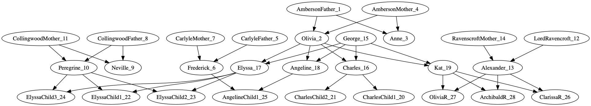
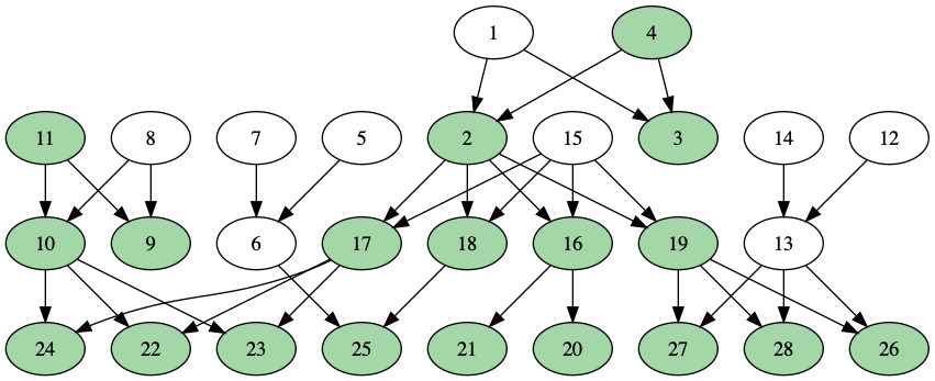
I start by marking the starting set of people as carriers of the trait. In the example below, only person #4 initially had the trait.

I find the carriers’ children, and mark them with the trait.

Then, I mark those children’s children with the trait also.

I repeat this process until all their descendants are marked:

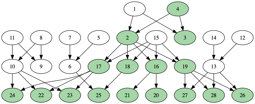
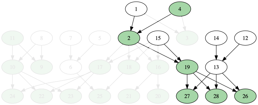
When I add more than one person to the starting set, I’ll have to watch for repeats.

In this next example, I’ve added person #11 to the starting set, so now I need to find the descendants of {#4, #11}. I have to be careful not to mark #24, #22, and #23 (on the left side of the graph) twice, since both their mother and their father have the trait:

After I verified that the procedure worked on small graphs, I ran the same algprithm on the entire 86-million node Familinx relations file.

Once I found all descendants of the original starting set, I exported the list of numerical IDs into the database. Then, I used a INNER JOIN to extract a list of profiles corresponding to the starting set:

create table profiles_bfsjoined as
select * from profiles inner join profileids_bfsout using (profileid);

This creates a new dataset, profiles_bfsjoined, containing only the profiles of the descendants.

I can then count the number of descendants alive per year, using the same query I used for the full dataset:

select count(1) from profiles_bfsjoined where birth_year is not null and death_year is not null
and birth_year > 1700 and birth_year <= 1809 and death_year >= 1809;

I can compare this with the number of people alive in the entire dataset to obtain the frequency of the trait in the population for that year.

Analysing the Familinx dataset

After counting the number of living descendants per year, a quick look at this graph shows that something is wrong: the expected exponential growth doesn’t happen.

The below graph shows the number of living descendants with the trait per year for all five starting ratios: all of them shows the population shrinking over time.

The relative frequency of people with the trait over time shows what looks like exponential decay for all starting ratios:

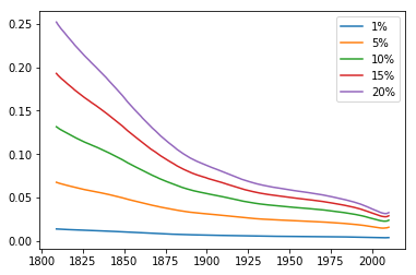
This contradicts our theory, which says that the ratio should be exponentially increasing. Why does this happen?

Well, maybe I screwed up the data processing. That’s definitely a possibility, although I’ve verified the code that marks descendants with a simpler graph (the one used above), and it worked fine. (If you find any errors, please let me know!)

Another possibility is that the Familinx dataset, as a genealogy database, is not suited for counting descendants because its bottom-up method of construction leaves out many descendants.

For example, take the simple family tree above. If I’m person 28 on this family tree, and I’m making a genealogy, I would care about my own ancestors, but I might not care much about my ancestors’ siblings (my aunts and uncles) and their descendants. So most of the family tree won’t be present in a genealogy database:

I haven’t had a chance to test this theory. I guess, to support or disprove this theory, I could try:

• counting the number of descendants starting from an ancestor and comparing it to what I expect
• start from a recent profile and working backwards, comparing expected number of aunts/uncles (from historical family size estimates) to actual number of aunts/uncles recorded.
• or ask someone with more experience working with the Familinx dataset. There’s a few sites such as @cureffi’s post that notes potential pitfalls for using the Familinx data.

Conclusion

I started this entire analysis to answer one question: if witchcraft spreads like a gene drive, then everyone should be a witch in a century and a half. What’s preventing that in Kat, Incorrigible’s world?

It took me way too long to realize the real answer:

Magic.

(duh.)

Seriously, though, there’s one common theme to everything in this article: test your assumptions.

1. I assumed that exponential growth should apply to the witchcraft population in the Kat books. So I tested that assumption with models, and concluded that this applies… in certain conditions
2. Unckless’s formulas assumed that the Selection Coefficient is low. Because I violated the assumption, I made a simulation to find how the formula would fail.
3. I assumed that indexes in SQL databases magically speeds things up. I tested it out, and it slowed things down instead.
4. I assumed that a genealogy database is a good way to track a person’s descendants. After I analyzed the data, it became clear that it doesn’t. I came up with a new set of assumptions to explain why, but now I’m looking for ways to challenge those new assumptions.
5. I assume that people want to read about kids’ books, population genetics, and PostgreSQL in the same article. The jury’s still out on this one ;)

So if you’re uncertain about an assumption, grab some data, write some code, or do an experiment!

My code can be found at my GitHub repository.

What I learned

• How Gene Drives work
• Population genetics models
• Theories’s predictions are only valid if their assumptions are met. Simulations can be used to validate the impact of violating assumptions.
• Simulating a Gene Drive’s spread
• Importing and exporting data from PostgreSQL
• How not to setup indexes in PostgreSQL
• Implementing a breadth-first search in Java
• Drawing graphs with Graphviz
• Why genealogy data can’t be used to estimate the number of descendants for a person

What I need to learn next

• How to optimize SQL indexes and queries
• Other experiments I can try with the Familinx data
• Other sources of open data I can play with
• How to write these blog posts in parts. (Seriously, this post, out of all the entries on this site, took me the longest to research and write.)
• How to draw fanart or write fanfiction, because nobody wants to read fancode.