Family Tree - Appendix
Appendix A: Gene drive math
Here’s how I adapted Unckless’s model of how gene drives spread for my representation of witchcraft as a gene drive.
By modifying and similifying the standard estimates for a Wright-Fisher model, Unckless arrived at the equation
q’ = (1 + Se)q
where
- q is the proportion of gene drive carriers in the population
- q’ is the rate of change of the proportion,
- Se is the selection coefficient, or how fast the gene drive spreads through the population.
The selection coefficient is given as
Se = hs(c - 1) + (1 - 2s)c
Where
- hs is the heterozygous fitness rate (how much reproductive advantage an organism gains if it only has one copy of the gene from gene drive)
- s is the homozygous fitness rate (how much reproductive advantage an organism gains if it only has one copy of the gene from gene drive)
- c is the conversion rate (the percentage of gene-drive carrying individuals that changes from having only one copy to having both copies of the gene drive, per generation)
For witchcraft, I assumed that witchcraft doesn’t give a reproductive advantage or a disadvantage to an individual, i.e.
hs = s = 0
I also assume that 100% of heterozygous individuals gets converted to homozygous in one generation, i.e.
c = 1.
This gives us a selection coefficient of
Se = 1
Subbing this into the original formula, we get
q’ = (1 + 1)q = 2q
After integrating, this simpifies to
q(t) = q0e2t
Where q0 is the initial ratio of gene drive carrying individuals.
This is obviously an exponential function, so I expect exponential growth of the number of witchcraft carriers.
With the conversion rate, we can now use Unckless’s other formula to predict how fast the gene drive would spread to half of the population, given a starting ratio:
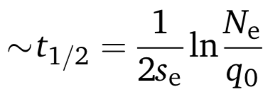
where
- Ne is the population size.
- q0 is the initial ratio, as before,
- Se is the selection coefficient, as before.
I’m using Ne = 2726151, to match the Familinx dataset’s 1809 population size.
Appendix B: Tweaking the simulation for other scenarios
What about the other assumptions we’ve made, such as constant population size?
Let’s try a variable number of offspring. Instead of making each pair have exactly two children, I randomly generated the number of children for each pair using a Poisson distribution, with mean = variance = 2.5 children/pair. Then I simulated the scenario again, with a starting population of 5000.
I got very similar results, suggesting that the exponential growth still holds even if the population is allowed to grow.
Simulations are easy to tweak, so trying new scenarios is simple. For example, I wondered what would happen if only one of a pair’s two children gets the trait. I changed two lines of code, and I got the result immediately.
Ah, exponential decline. That was easy.